This page was generated by nbsphinx from docs/notebooks/phys180e/phys180e_example.ipynb.

Accessing Data from a Physics 180E HDF5 File

%matplotlib inline

import numpy as np
import matplotlib.pyplot as plt

from pathlib import Path

from bapsflib import phys180E

plt.rcParams.update(
    {"figure.figsize": [10, 0.6 * 10], "font.size": 16}
)

Let’s define the file name and path to the HDF5 file.

# _HERE is the location of this jupyter notebook
_HERE = Path.cwd()
_FILENAME = "sample_phys180e_axial_bdot.hdf5"
_FILE = (_HERE / _FILENAME).resolve()

print(
    f"File name & path: {_FILE}\n"
    f"File exists: {_FILE.exists()}"
)

File name & path: /home/docs/checkouts/readthedocs.org/user_builds/bapsflib/checkouts/latest/docs/notebooks/phys180e/sample_phys180e_axial_bdot.hdf5
File exists: True

The HDF5 file can now be opened using the File class on phys180e.

f = phys180E.File(_FILE)

/home/docs/checkouts/readthedocs.org/user_builds/bapsflib/envs/latest/lib/python3.14/site-packages/bapsflib/_hdf/maps/digitizers/templates.py:532: HDFMappingWarning: `config_name` not specified, assuming 'lecroy'.
  warn(
/home/docs/checkouts/readthedocs.org/user_builds/bapsflib/envs/latest/lib/python3.14/site-packages/bapsflib/_hdf/maps/digitizers/templates.py:612: HDFMappingWarning: No `adc` specified, but only one adc used...assuming adc 'lecroy'
  warn(

f is now an object instance of the phys180e.File class. All the functionality provided by the File class is accessible via dot access.

For example, a summary of the digitizer can shown by…

f.digitizers

{'LeCroy_scope': <bapsflib._hdf.maps.digitizers.lecroy.HDFMapDigiLeCroy180E object at 0x7d725403d6a0>}

| Digitizer      | Configuration | ADC      | (board, [channel, ...]) | Shot Num. Range | nt   |
+----------------+---------------+----------+-------------------------+-----------------+------+
| 'LeCroy_scope' | 'lecroy'      | 'lecroy' | (0, (1, 2, 3, 4))       | ??              | 2500 |

Here, the digitizer used to recorded data was the 'LeCroy_scope' and all 4 channels recorded data with a record length of 2500.

And a more details digitizer report can be accessed on the overview attribute.

f.overview.report_digitizers()

Digitizer Report
^^^^^^^^^^^^^^^^

LeCroy_scope (main)
+-- adc's:  ('lecroy',)
+-- Configurations Detected (1)                               (1 active, 0 inactive)
|   +-- lecroy                                                active
|   |   +-- adc's (active):  ('lecroy',)
|   |   +-- path: /Acquisition/LeCroy_scope
|   |   +-- lecroy adc connections
|   |   |   |   +-- (brd, [ch, ...])               bit  clock rate   nshotnum  nt        shot ave.  sample ave.
|   |   |   |   +-- (0, (1, 2, 3, 4))              None None         50        2500      None       None

Reading Digitizer Data

Digitizer data can be retrieved by using the read_data() method.

For example, lets retrieve all the recorded data for channel 2 of the digitizer.

data = f.read_data(board=0, channel=2, silent=True)
data.dtype

dtype([('shotnum', '<u4'), ('signal', '<f4', (2500,)), ('xyz', '<f4', (3,))])

The retrieved data has three fields:

• "shotnum": This is the shot number array.

• "signal": This is the recorded signal data.

• "xyz": This field contains probe positions. However, we have not read out any position data, so this will be covered later in the notebook.

The total number of shots for this HDF5 file is…

data["shotnum"].size

50

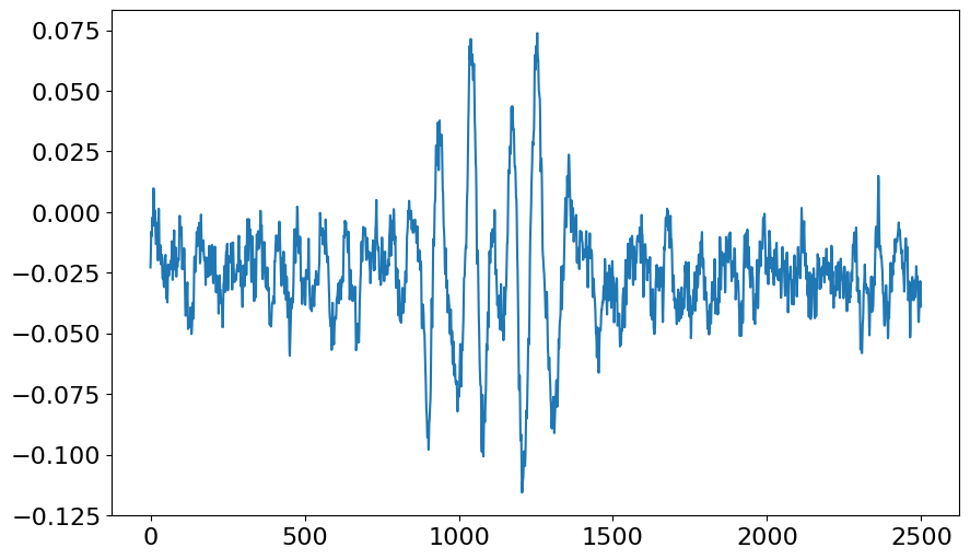
Let’s say we wanted to plot the signal for shot number 49. We could do something like…

mask = data["shotnum"] == 49
data49 = data["signal"][mask, ...]

The ellipses ... is requires since data["shotnum"] (and thus mask) have a shape of (50,), where as data["signal"] has a shape of (50, 2500).

plt.plot(data49.squeeze());

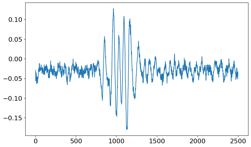
A single record can also be read directly by read_data().

data35 = f.read_data(0, 2, shotnum=35, silent=True)

plt.plot(data35["signal"].squeeze());

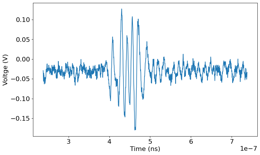
Reading the Time Series

The File object also provides a convienece method, get_time_array(), to retrieve the time array associated with the digitized data. This method takes just one argument, the data array.

# let's just work with data35 from now on
data = data35

# get the time array
time = f.get_time_array(data)

plt.plot(time, data["signal"].squeeze())
ax = plt.gca()
ax.set_xlabel("Time (ns)")
ax.set_ylabel("Voltge (V)");

The time array can also be retrieved before any data is extracted.

digitized_info = f.get_digitizer_specs(0, 2, silent=True)
time_from_digi_info = f.get_time_array(digitized_info)

# see... both arrays are equal
np.allclose(time, time_from_digi_info)

True

Reading Position Information

The digitized data is often associated with a probe that is connected to an automated probe drive (or a control device). This probe drive also records this position data in the HDF5 file. Similarly to f.digitizers, f.controls will yield a brief summary of the mapped control devices…

f.controls

{'180E_positions': <bapsflib._hdf.maps.controls.positions180e.HDFMapControlPositions180E object at 0x7d725403d7f0>}

| Control          | Configuration | Shot Num. Range | Readout Data Fields |
+------------------+---------------+-----------------+---------------------+
| '180E_positions' | 'positions'   | ??              | ('xyz',)            |

Here the control device is call "180E_positions" and will map to the "xyz" field briefly mentioned when discussing the extracted digitizer data.

A more detailed report can also be displayed using the overview attribute.

f.overview.report_controls()

Control Device Report
^^^^^^^^^^^^^^^^^^^^^

180E_positions
+-- path:     /Control/Positions
+-- contype:  ConType.MOTION
+-- Configurations Detected (1)
|   +-- positions
|   |   +-- {'dset paths': ('/Control/Positions/positions_setup_array',),
|   |   +--  'shotnum': {'dset field': ('Line_number',),
|   |   +--              'dset paths': ('/Control/Positions/positions_setup_array',),
|   |   +--              'dtype': <class 'numpy.int32'>,
|   |   +--              'shape': ()},
|   |   +--  'state values': {'xyz': {'config column': None,
|   |   +--                           'dset field': ('x', 'y', ''),
|   |   +--                           'dset paths': ('/Control/Positions/positions_setup_array',),
|   |   +--                           'dtype': <class 'numpy.float64'>,
|   |   +--                           'shape': (3,)}}}

Retrieving the control data can be done using the read_control() method.

cdata = f.read_controls(["180E_positions"], silent=True)
cdata.dtype

dtype([('shotnum', '<u4'), ('xyz', '<f8', (3,))])

The retrieved control data has two fields:

• "shotnum": This is the shot number array.

• "xyz": This field contains probe positions.

So, the position for shot number 35 is…

print(
    f"Shot number: {cdata['shotnum'][34]}\n"
    f"Position [x, y, z]: {cdata['xyz'][34]}"
)

Shot number: 35
Position [x, y, z]: [-39. -10.   0.]

Now, this is not so convenient since the position data is not paired with the signal data. So, read_data provides a mechanism for mating the digitizer and position data at the same time.

all_data = f.read_data(0, 2, add_controls=["180E_positions"], shotnum=35, silent=True)

All the extracted data in all_data is the same as what we have extracted before.

print(
    f"Shot number is the same: {np.allclose(data['shotnum'], all_data['shotnum'])}\n"
    f"Signal data is the same: {np.allclose(data['signal'], all_data['signal'])}\n"
    f"Position data is the same: {np.allclose(cdata['xyz'][34], all_data['xyz'])}\n"
)

Shot number is the same: True
Signal data is the same: True
Position data is the same: True

Close the File instance

The File instance will automatically close itself when Python garbage collects at the close of this notebook. However, it is good practice to explicitly close the file.

f.close()